

AVERAGEIFS Function (LibreOffice Calc)
The AVERAGEIFS function in LibreOffice Calc calculates the average of values that meet multiple conditions across one or more ranges. This guide explains syntax, operators, wildcards, examples, errors, and best practices.
Verification status: Consult the documentation and examples below. Native application testing has not been documented for this guide. How formula examples are checked
Native-tested visual example: Average completed team scores
Quick answer: Exclude other teams and pending measurements. The following example was run in LibreOffice Calc 25.2.3.2, not simulated or inferred from a formula description.
Enter the sample data
The downloadable workbook uses these exact rows on its Example sheet. Enter the values or download the editable AVERAGEIFS ODS practice workbook instead.
| Sheet row | A: Record | B: Team | C: Status | D: Score |
|---|---|---|---|---|
| 5 | T-01 | Alpha | Complete | 80 |
| 6 | T-02 | Beta | Complete | 60 |
| 7 | T-03 | Alpha | Complete | 90 |
| 8 | T-04 | Alpha | Pending | 70 |
| 9 | T-05 | Alpha | Complete | 100 |
| 10 | T-06 | Beta | Pending | 95 |
Formula and result
Select E5 in the practice workbook. The formula is:
=AVERAGEIFS(D5:D10;B5:B10;"Alpha";C5:C10;"Complete")
Verified output: 90. Only scores 80, 90 and 100 satisfy both tests, giving an average of 90.
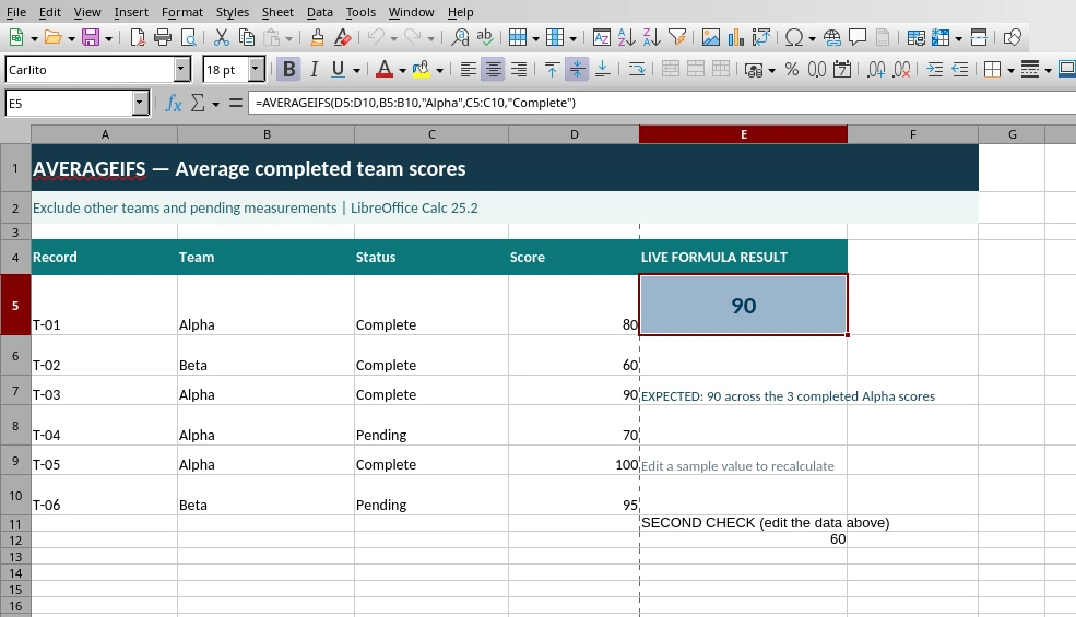
Screenshot captured from LibreOffice Calc 25.2.3.2. The formula, input values and E5 result are visible in the actual application.
Second example you can try
The workbook also includes this independently tested variation in E12:
=AVERAGEIFS(D5:D10;B5:B10;"Beta";C5:C10;"Complete")
Verified output: 60. Change the related input cell and press Enter to see the result update.
Common mistake: If no rows match, AVERAGEIFS returns a division-by-zero error; criteria ranges must match the average-range size.
Official documentation: LibreOffice Calc reference for AVERAGEIFS. Test scope: These two worked examples were recalculated in Calc 25.2.3.2; other historical formulas elsewhere on this page may still require separate testing. This file includes no generated or artificial application screenshot.
What the AVERAGEIFS Function Does
- Averages values that satisfy two or more conditions
- Supports numeric, text, date, logical, and wildcard criteria
- Allows conditions across multiple ranges
- Requires all criteria ranges to be the same size
- Ignores empty cells automatically
- Ideal for multi‑condition reporting and analytics
AVERAGEIFS is the multi‑condition extension of AVERAGEIF.
Syntax
AVERAGEIFS(average_range; criteria_range1; criteria1; criteria_range2; criteria2; ...)
Basic Examples
Average values where Region = “North” AND Sales > 1000
=AVERAGEIFS(C1:C100; A1:A100; "North"; B1:B100; ">1000")
Average values between 50 and 100
=AVERAGEIFS(B1:B100; A1:A100; ">=50"; A1:A100; "<=100")
Average values where Status = “Open” AND Priority = “High”
=AVERAGEIFS(C1:C100; A1:A100; "Open"; B1:B100; "High")
Average values where Date is in 2025 AND Category = “A”
=AVERAGEIFS(C1:C100; A1:A100; ">="&DATE(2025;1;1); A1:A100; "<"&DATE(2026;1;1); B1:B100; "A")
Text & Wildcard Examples
Average values where text starts with “A”
=AVERAGEIFS(B1:B100; A1:A100; "A*")
Average values where text contains “car”
=AVERAGEIFS(B1:B100; A1:A100; "*car*")
Average values where text ends with “ing”
=AVERAGEIFS(B1:B100; A1:A100; "*ing")
Case‑sensitive conditional average
AVERAGEIFS is case‑insensitive.
For case‑sensitive logic, use SUMPRODUCT:
=SUMPRODUCT((EXACT(A1:A100; "Apple")) * B1:B100)
  / SUMPRODUCT(EXACT(A1:A100; "Apple"))
Advanced Examples
Use cell references as criteria
=AVERAGEIFS(C1:C100; A1:A100; "=" & D1; B1:B100; ">=" & E1)
Average values between two cell values
=AVERAGEIFS(C1:C100; A1:A100; ">=" & D1; A1:A100; "<=" & E1)
Average values where another column is not blank
=AVERAGEIFS(C1:C100; A1:A100; "<>")
Average across sheets
=AVERAGEIFS(Sheet1.C1:C100; Sheet1.A1:A100; "North")
+ AVERAGEIFS(Sheet2.C1:C100; Sheet2.A1:A100; "North")
Average errors (rare but possible)
=AVERAGEIFS(B1:B100; A1:A100; "#N/A")
OR logic using AVERAGEIFS
=AVERAGEIFS(C1:C100; A1:A100; "North")
+ AVERAGEIFS(C1:C100; A1:A100; "South")
Complex OR/AND logic using SUMPRODUCT
=SUMPRODUCT(((A1:A100="North") + (A1:A100="South")) * (B1:B100>1000) * C1:C100)
  / SUMPRODUCT(((A1:A100="North") + (A1:A100="South")) * (B1:B100>1000))
Common Errors and Fixes
Err:504 — Parameter error
Occurs when:
- Ranges are different sizes
- Criteria is malformed
- Semicolons are incorrect
AVERAGEIFS returns 0 unexpectedly
Possible causes:
- Criteria missing quotes
- Numbers stored as text
- Hidden spaces or non‑breaking spaces
- Wildcards used incorrectly
Fix:
Check with:
=LEN(A1)
AVERAGEIFS returns #DIV/0!
Occurs when:
- No values match the conditions
- All matching values are empty
AVERAGEIFS is slow on large datasets
Use:
- Named ranges
- Helper columns
- Database functions (DAVERAGE) for structured data
AVERAGEIFS does not support OR logic natively
Use multiple AVERAGEIFS or SUMPRODUCT.
Best Practices
- Ensure all ranges are the same size
- Always quote criteria containing operators
- Use cell references for dynamic criteria
- Use AVERAGEIF for single‑condition logic
- Use SUMPRODUCT for advanced OR/AND combinations
- Clean imported data before applying criteria
Reproducible example (tested in LibreOffice Calc)
This standalone example was calculated in LibreOffice Calc 25.2.3.2 and matched the expected value. It is a practical cross-check of one usage, not proof that every example elsewhere on this page is correct.
Use this small practice sheet for the ranges referenced in the formula:
| Row | A (Quantity) | B (Amount) | C (Category) |
|---|---|---|---|
| 1 | 1 | 10 | apple |
| 2 | 2 | 20 | pear |
| 3 | 3 | 30 | apple |
| 4 | 4 | 40 | pear |
| 5 | 5 | 50 | apple |
=AVERAGEIFS(B1:B5;C1:C5;"apple")
Expected result: 30.
Average amounts where the corresponding category is apple.
If the result differs, check the referenced cells, argument separators and number formatting. For more information, consult the LibreOffice Calc official help.