Highlight an Entire Row by Status in LibreOffice Calc

Select the table’s data rows and create a Formula is conditional format. For a table starting at A2 whose status is in column D, use $D2="Blocked". The dollar sign fixes column D; the unfixed row number lets each row test its own status.

This colors the selected cells across a row. It does not need to format every column of the spreadsheet, and it does not record when the status changed.

Requirements and sample

Use desktop Calc with Data → Calculate → AutoCalculate enabled. These steps follow the standard menu bar and current LibreOffice 26.8 Help; the tabbed interface places conditional formatting under Home → Conditional. Save as ODS to retain the rule.

Enter the following in A1:D5, or open the status-tickets CSV. The CSV contains data, not formatting rules.

Ticket	Owner	Amount	Status
T-101	Alex	92	New
T-102	Morgan	105	Blocked
T-103	Sam	130	Done
T-104	Alex	87	Blocked

The target is to highlight A3:D3 and A5:D5. The header and the other two records should keep their usual appearance.

1. Add the row rule

1. Click A2 and select through D5, or enter A2:D5 in the Name Box. Do not include row 1.
2. Choose Format → Conditional → Condition → More rules to open the full dialog in Calc 26.8.1.1. Versions without that submenu may open the dialog directly from Condition.
3. Set the condition type to Formula is and enter $D2="Blocked" in the expression box. Use straight double quotes around Blocked.
4. Under Apply Style, choose New Style. Name it Blocked pale red, give it a pale red background with readable dark text, and confirm the style.
5. Check that the dialog’s Range is A2:D5, then confirm.

The conditional-formatting dialog applies a cell style when the condition succeeds. Formula is evaluates a logical expression rather than comparing each target cell’s own text with Blocked.

Select a screenshot to open the full-size image.

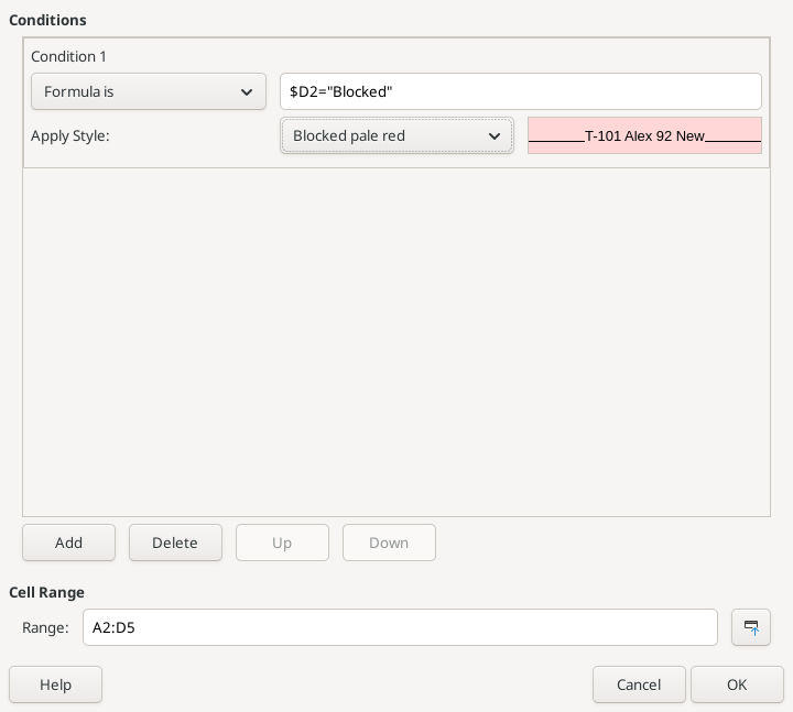
Native LibreOffice Calc 26.8.1.1 on Linux, captured 16 October 2026. The status column is fixed while the row remains relative.

Checkpoint: eight cells should be highlighted: four across row 3 and four across row 5. If only the two status cells change, the range probably contains only D2:D5.

2. Prove that the rule follows the status

1. Change D2 from New to Blocked. A2:D2 should gain the style.
2. Change D3 from Blocked to Done. A3:D3 should lose the conditional style.
3. Leave row 5 unchanged. The highlighted records should now be T-101 and T-104.
4. Restore the original statuses if you want to repeat the example.

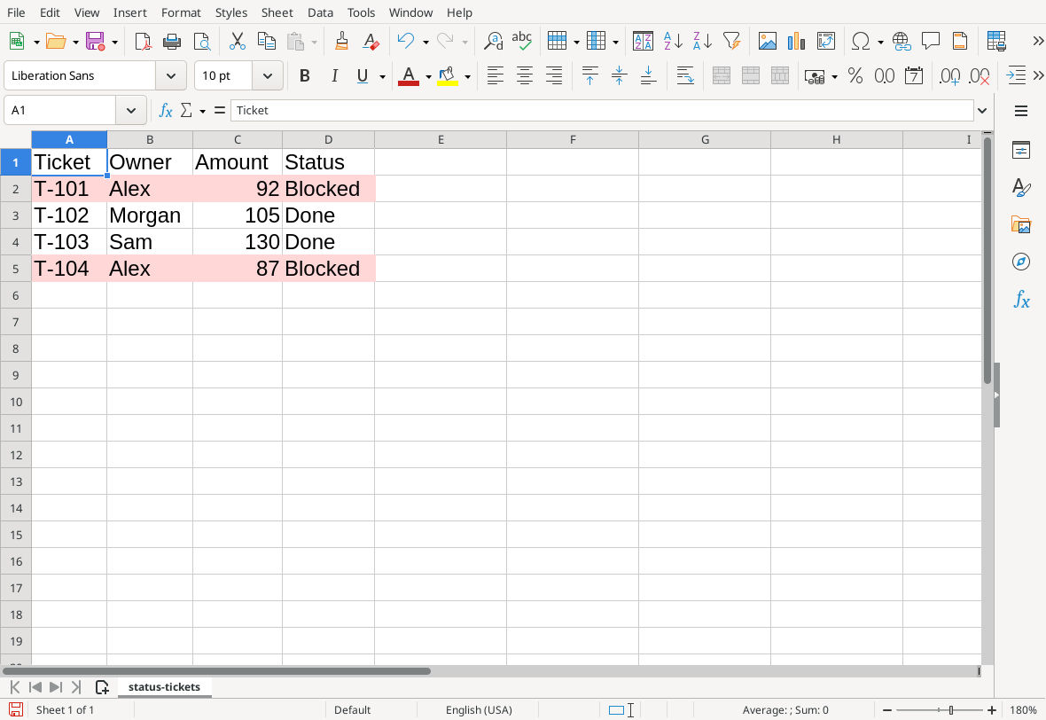
LibreOffice Calc 26.8.1.1: changing the statuses moves the row highlighting without manual fill changes.

No manual fill change is required. Calc reevaluates the condition when the values change, provided AutoCalculate is enabled. See Applying Conditional Formatting.

Why $D2 works and $D$2 does not

The rule is written for the top-left data cell, A2. Across that row, every target must examine D2. Down one row, every target must examine D3.

Reference in the rule	Effect
$D2	Fix column D; let the row change. Correct for this layout.
$D$2	Every record checks D2. One status can color the whole selected block.
D2	The column can shift as the rule is applied across the row.
$D1	Tests the preceding row because the target range begins at row 2.

For a table beginning at A7, write $D7="Blocked" instead. If the status moves to F, use $F7="Blocked". The formula must agree with both the first target row and the actual status column. This follows Calc’s absolute and relative reference model.

3. Extend or refine the rule

When adding records below row 5, open Format → Conditional → Manage, select the existing format, and edit its Range to A2:D20 or the real last row. Keep $D2="Blocked" because the range still starts at row 2. An explicit range extension is easier to audit than assuming every paste will carry the rule correctly.

To add a second status color, add a condition in that same format, such as $D2="Done", and choose a different style. Calc evaluates the list in order and uses the first matching condition. Manage lists the first rule for each range, so open it to inspect additional conditions. Avoid creating overlapping ranges unintentionally. See Manage Conditions.

For a combined test, use AND($D2="Blocked";$C2>100). In the original sample only row 3 qualifies. This example uses English function names and semicolon argument separators; use your configured names and separator if they differ. See AND.

Keep the simpler value-only rule when it fits

If you only need to highlight numbers greater than 100, a row formula is unnecessary. On a separate practice sheet, enter 92, 105, 130, 87 in B2:B5. Select that range, choose Cell value is → is greater than, enter 100, and apply a style. Only 105 and 130 should change. This preserves a useful distinction: value conditions act on each selected cell, whereas the status formula deliberately points to another column. See Cell value is.

Troubleshooting

• One row is out of step: compare the first row in Range with the row number in the formula.
• Everything changes together: remove the dollar sign before the row number, not the one before D.
• Nothing changes: check AutoCalculate, the exact status text, the range and the style’s background. In an unused cell, =D3="Blocked" helps test the comparison separately.
• A pasted status looks right but fails: inspect spaces. TRIM helps with ordinary leading/trailing spaces. If capitalization must be exact, test EXACT($D2;"Blocked"); see EXACT.
• Manual fill seems ignored: a matching conditional style takes visual precedence. The underlying manual formatting remains and becomes visible when no condition matches.
• New rows stay plain: inspect Range in Manage rather than repeatedly adding new overlapping formats.

Before distributing an XLSX copy, reopen it and repeat the two-status-change test in the receiving application. This guide’s rule is a current-state indicator; tracking the time of a change requires a separate history or logging design.

Verification: the single-status formula rule, both sets of highlighted rows and saved-file reopening were tested in LibreOffice Calc 26.8.1.1 on Linux (English interface) on 16 October 2026. The screenshots are native captures. Additional rule variations and cross-format caveats are documentation-based; their expected matches were checked independently.