Fix a LibreOffice Calc Pivot Table That Misses New Rows

If new rows are missing from a Calc pivot table, check the source range before refreshing again. A pivot based on A1:C9 does not include a record appended in row 10. Select the pivot, choose Data → Pivot Table → Insert or Edit, and extend its Source to include that row. Confirm the layout; use Data → Pivot Table → Refresh to update the summary after later source edits.

Refresh recalculates the pivot from its configured source. It is not a guarantee that data appended outside a fixed range will become part of that source.

Requirements and practice data

Use desktop LibreOffice Calc with the standard menu bar. The steps follow current 26.8 Help. Work in an ODS copy so the pivot and its source remain in one workbook; CSV cannot store pivot tables or additional sheets.

Download the feature-practice sales CSV. Open it as comma-separated UTF-8 text, check that Amount imports as numbers, and rename its sheet Sales. The eight records occupy A2:C9 beneath one header row:

Region	Channel	Amount
North	Online	120
North	Retail	80
South	Online	90
South	Retail	140
North	Online	60
South	Online	30
North	Retail	40
South	Retail	20

Do not add a source grand-total row. A pivot already calculates totals, and a total included as a record would double-count the amounts.

1. Build a pivot with a known starting range

1. Select Sales.A1:C9 explicitly, including the three headers.
2. Choose Insert → Pivot Table. In Select Source, choose Current selection and confirm. The standard Data → Pivot Table → Insert or Edit command is another documented entry point.
3. Drag Region into Row Fields, Channel into Column Fields, and Amount into Data Fields.
4. Confirm the data field uses Sum, not Count. Double-click its button in Data Fields if you need to change the aggregation.
5. Expand Source and Destination if necessary. Check that Source covers $Sales.$A$1:$C$9, then choose New sheet as the destination. Leave room for a growing pivot rather than putting it over other data.
6. Keep totals enabled and confirm the dialog.

The Pivot Table dialog documentation describes the field areas, source controls and new-sheet destination. A destination on occupied cells can overwrite their contents.

Checkpoint: the starting summary should be:

Region	Online	Retail	Total
North	180	120	300
South	120	160	280
Grand total	300	280	580

North/Online is 120 + 60 = 180; South/Retail is 140 + 20 = 160. Check both individual groups and the grand total: a correct overall sum can conceal records assigned to the wrong category.

2. Reproduce the missing-row problem

1. Return to Sales and enter North, Online, 50 in A10:C10. This is a ninth data record, outside the original range.
2. Click a cell inside the pivot and choose Data → Pivot Table → Refresh.
3. Compare the total with the complete source. =SUM(Sales.C2:C10) in a spare cell should return 630.
4. If the pivot still shows 580, inspect its source boundary. If it already shows 630 because your actual source definition expanded, check that its source now includes row 10; there is no need to force a failure.

The explicit refresh command is documented in Updating Pivot Tables. For comparison, changing a value inside A2:C9 and refreshing does not require an expanded boundary.

3. Expand the source, then verify the new result

1. Click a cell inside the pivot and choose Data → Pivot Table → Insert or Edit to reopen its layout. Right-clicking a pivot cell and choosing Properties is an alternative documented in Editing Pivot Tables.
2. Expand Source and Destination. For a selection-based source, replace the old range with $Sales.$A$1:$C$10, or use the range picker to select A1:C10 on Sales. Keep the header row.
3. Check the existing field arrangement and destination before confirming. You are editing the current pivot, not creating another summary on top of it.
4. Confirm the dialog. In the tested Calc 26.8.1.1 workflow, confirming the expanded source recalculated the pivot immediately. An additional Data → Pivot Table → Refresh retained the same result; it was not required to make the source edit take effect. Compare these figures.

Select a screenshot to open the full-size image.

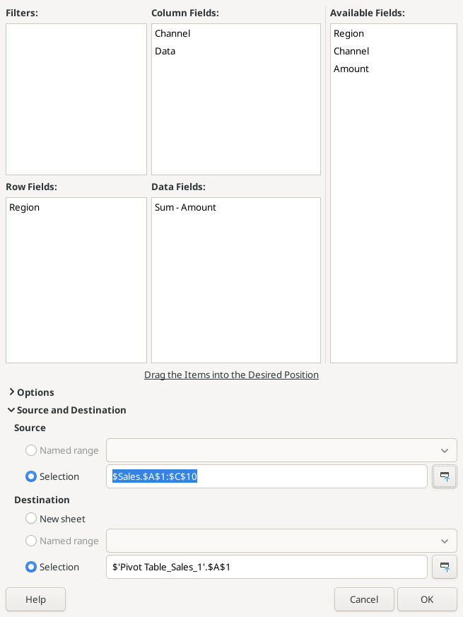
Native LibreOffice Calc 26.8.1.1 on Linux, captured 16 October 2026. Change the Source selection, not the output destination.

Region	Online	Retail	Total
North	230	120	350
South	120	160	280
Grand total	350	280	630

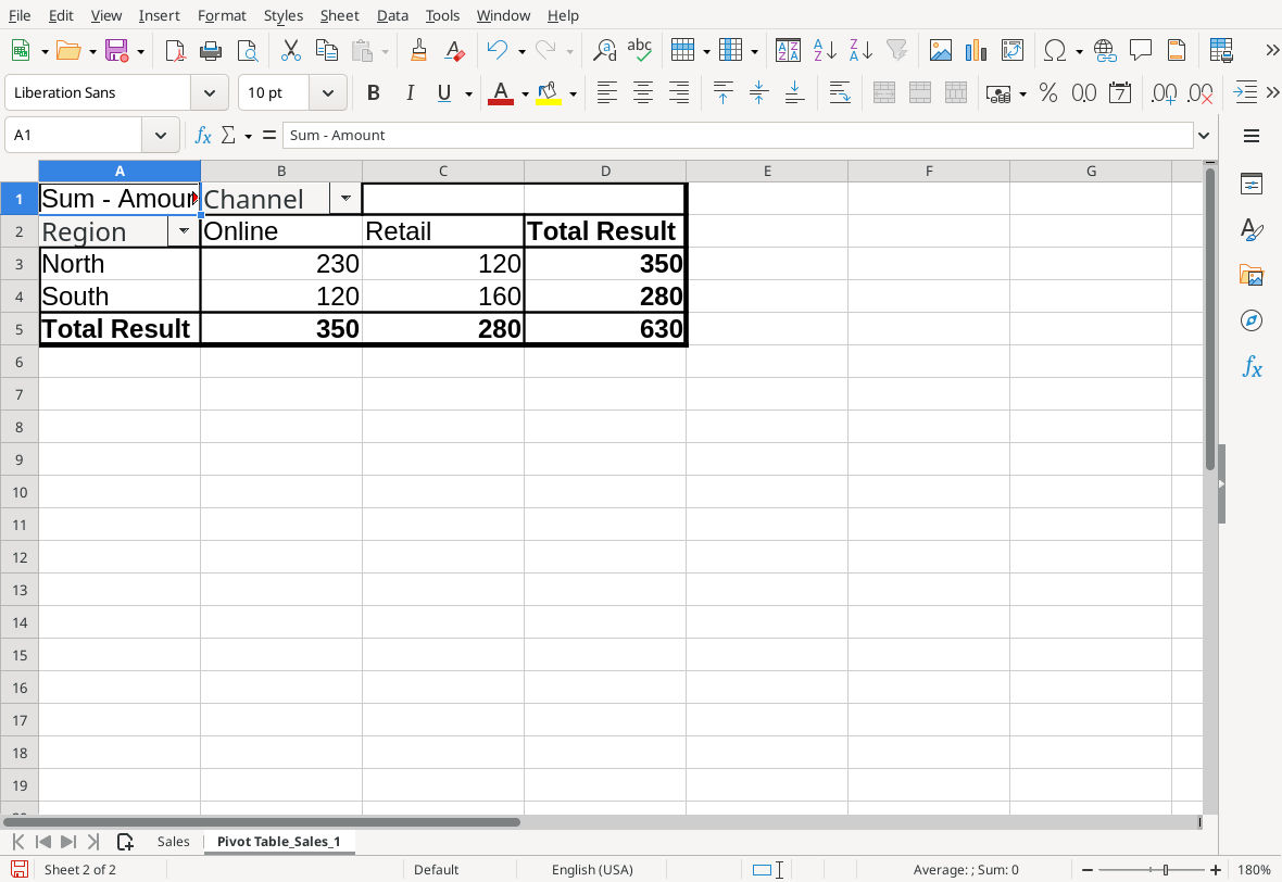
LibreOffice Calc 26.8.1.1: the newly included North/Online record raises the grand total to 630.

Only North/Online gains 50. If South or Retail changes, review the appended record and field layout. If the grand total is 630 but North/Online is still 180, look for a second label such as North with a trailing space.

Why this fixes the problem

There are three separate things to maintain: the actual records, the definition telling the pivot where those records are, and the pivot’s calculated output. Appending a record changes the first; editing Source changes the second; refreshing updates the third. Repeatedly doing only the final step cannot repair a source definition that still excludes the new record.

For recurring imports, a named range can make the boundary easier to find. However, a name defined as A1:C9 is still a fixed range until its definition changes. Inspect the pivot’s selected source name and the name’s actual extent; do not assume naming it makes it dynamic.

If records are still missing

• Source includes row 10, but the result is still 580: click inside the intended pivot before refreshing. A workbook may contain several similar summaries.
• Grand total is 9 or another record count: the data field may use Count. Choose Sum and inspect text-formatted amounts. Numeric-looking text should be corrected at import rather than hidden by changing only its display format.
• A valid source record is excluded: inspect the pivot’s field/filter selections. Restore all wanted categories before reconciling the result.
• A region appears twice: compare the source labels character by character. TRIM helps clean ordinary extra spaces; refresh after fixing labels.
• The range stops before an internal gap: select the complete rectangular source explicitly. Clicking one cell is less reliable than selecting A1 through the true final row and column.
• Source is a registered database rather than cells: update the actual data source and its query/import first. A local cell-range edit is not the right repair for that connection type.

Avoid whole-column sources as a reflexive fix: they can bring blank records, unrelated future data and unnecessary processing into the summary. Use a deliberate boundary and include a source-range check in the import routine.

Final reconciliation

Check 630 with SUM and one category with SUMIFS, for example =SUMIFS(Sales.C2:C10;Sales.A2:A10;"North";Sales.B2:B10;"Online"), which should return 230. The formula uses English names and semicolon separators; adapt those to your Calc configuration.

Save, reopen and repeat the checks. After importing an Excel pivot table, refresh it in Calc as recommended by LibreOffice Help; cross-format behavior should be tested in the application that will consume the result.

Verification: in LibreOffice Calc 26.8.1.1 on Linux (English interface), refresh of the fixed A1:C9 source stayed at 580 after the append. Expanding the source through row 10 produced 630 and the group totals shown above. The test and native screenshots were made on 16 October 2026; both matrices were also checked independently. Close/reopen persistence, database sources and cross-format cases were not tested natively.