

GETPIVOTDATA in FreeOffice PlanMaker: Syntax and Worked Examples
Retrieve grand totals and field-item intersections from a genuine PlanMaker pivot table with GETPIVOTDATA.
Verification status: See the evidence and test scope described in this guide. How formula examples are checked
Quick answer
GETPIVOTDATA retrieves an aggregated value from an existing pivot table. A source-data range, manually typed summary or copied pivot-looking table is not a substitute for that pivot structure.
For a genuine pivot whose Values area sums Amount, =GETPIVOTDATA("Amount",E2) requests its grand total, provided E2 is a cell inside that pivot report. Adding field/item pairs narrows the requested aggregate.
Syntax and required context
=GETPIVOTDATA(ValueField, PivotRange [, Field1, Label1, Field2, Label2, ...])
ValueField is the name of the field placed in the pivot’s Values area, quoted as text. PivotRange can be a reference to any cell in the target pivot report; it is not quoted. Optional field names and item labels are supplied as quoted pairs.
Use actual field and item names from the pivot. The function does not infer that a column called Revenue is equivalent to Amount, or that a source cell outside the pivot report identifies the pivot.
Step-by-step: a fictional regional report
Enter this source table in A1:C5:
| Region | Product | Amount |
|---|---|---|
| North | A | 10 |
| North | B | 20 |
| South | A | 30 |
| North | A | 5 |
Create a genuine pivot table from the source, with Region and Product as row fields and Amount in Values using Sum. Place the report so its target range includes E2. Do not merely type the totals into E:G.
The source records independently sum to 65. North totals 35 and South 30. Within North, Product A totals 15 and Product B 20. With that actual pivot context, the expected queries are:
| Formula | Independent aggregate |
|---|---|
=GETPIVOTDATA("Amount",E2) |
65 |
=GETPIVOTDATA("Amount",E2,"Region","North") |
35 |
=GETPIVOTDATA("Amount",E2,"Region","South") |
30 |
=GETPIVOTDATA("Amount",E2,"Region","North","Product","A") |
15 |
=GETPIVOTDATA("Amount",E2,"Region","North","Product","B") |
20 |
The repeated North/A source rows are aggregated together. The two field/item pairs describe an intersection, not a sum of separate North and A totals.
Advanced use: stable report queries
A direct reference to a displayed total, such as a particular cell in a pivot report, describes a physical location. GETPIVOTDATA describes a requested field/item aggregate within an identified pivot. Keep the reference inside the report and maintain the field names when redesigning the layout.
The help permits a named range as PivotRange if you explicitly define it for the report. The pivot object’s automatically generated name, such as “Pivot table 1,” is not automatically such a worksheet name. The reference points to the named-area tools for creating an actual named range. This guide’s native cases use a plain cell reference, not an untested name setup.
A pivot aggregation can be changed from Sum to another summary operation. The interpretation of the retrieved value depends on the actual Values configuration. A numeric result alone does not prove that the pivot uses the intended aggregation or reflects the latest source-data edits.
Missing items and invalid references
The short official page does not enumerate every error for a missing item, misspelled field, filtered-out combination or non-pivot reference. The bounded native cases include a missing Region item and an ordinary source cell as PivotRange; both returned #REF! in the tested build, as detailed below.
Check the pivot’s source, aggregation and visible structure before treating an unexpected result as a formula bug. Preserve the genuine pivot object in the workbook when sharing a query; a values-only copy of its displayed cells does not establish equivalent behavior.
Compatibility and scope
The reference documents the function but does not establish its original introduction release or a universal file-format roundtrip. The native workbook retained an actual pivot definition and cache as well as formulas and outputs. The source arithmetic independently checks the retrieved aggregates.
Native pivot results
A genuine pivot was created in FreeOffice PlanMaker 2024 revision F1238.1005 with Region and Product row fields and Amount summed in Values. The report starts at E2 and displays the caption Sum of Amount. The formulas successfully used the source field name “Amount”, as shown in the examples.
The grand total and four selected aggregates returned 65,35,30,15,20. The missing Region item and the ordinary source-cell reference A1 both returned #REF!. All seven expressions, the fifteen source cells including headers, and the genuine pivot definition/cache were retained after native PMDX save and reopen. This confirms the specified pivot context, not arbitrary field naming, filtering or file-format behavior.
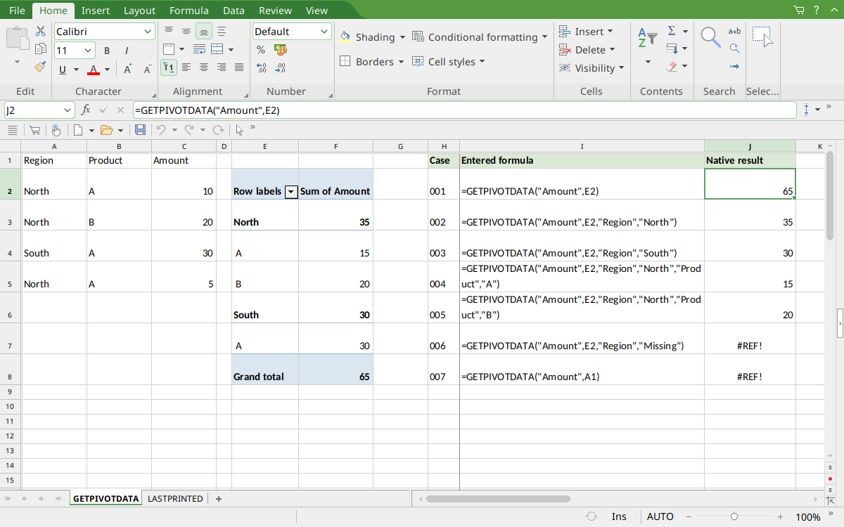
Selected J2 displays 65 and its formula bar references E2. The actual pivot is visible in E:F, including North 35, South 30 and grand total 65. J3:J6 display 35,30,15,20; J7:J8 show #REF! for the two invalid-context queries. Longer two-pair formula labels wrap within column I.
Version and verification scope
The official FreeOffice PlanMaker 2024 reference was checked October 18, 2026. The installed application is FreeOffice PlanMaker 2024 revision F1238.1005. The original introduction version is not established by this evidence; the current reference does not identify the function as deprecated or retired. No availability claim for a different edition or a 2026 release is implied.
The seven native formulas were calculated against the genuine pivot described above and retained after PMDX save and reopen. Named-range setup, other aggregation operations and Excel file exchange were not tested. English formulas in this guide use commas; use the separators required by your formula settings.