

PlanMaker TREND Function: Calculate fitted and predicted values from a straight line
Fit and evaluate a least-squares line with TREND in FreeOffice PlanMaker 2024, including defaults and forced-zero intercepts.
Verification status: See the evidence and test scope described in this guide. How formula examples are checked
Quick answer: for x values 1, 2, 3, 4 and y values 3, 5, 6, 9, least squares gives the fitted line y=1.9x+1. TREND predicts 10.5 at x=5 and 12.4 at x=6.
Syntax and optional arguments
=TREND(y_values [, x_values] [, New_x_values] [, Constant])
y_values contains dependent observations. x_values supplies the corresponding independent coordinates; if omitted, PlanMaker uses 1, 2, 3, and so on. New_x_values specifies where to evaluate the fitted line. If omitted, the existing x coordinates are used.
Constant defaults to TRUE, which estimates an intercept. FALSE forces the intercept to zero and adjusts the slope accordingly. It does not simply subtract an already fitted intercept while leaving the slope unchanged.
TREND returns an array of fitted or predicted y values. The official reference calls for array-formula entry. The controls below inspect elements with INDEX; they do not establish array-entry shortcuts or automatic spill behavior in the interface.
Enter a non-perfect dataset
| Row | A: Existing x | B: Observed y | C: New x |
|---|---|---|---|
| 2 | 1 | 3 | 5 |
| 3 | 2 | 5 | 6 |
| 4 | 3 | 6 | |
| 5 | 4 | 9 |
Enter =INDEX(TREND(B2:B5,A2:A5,C2:C3),1,1) outside the data grid to read 10.5. Change the INDEX row to 2 to read 12.4. The new-x column contains two values, so the mathematical output is a two-element column.
The observed values are not perfectly collinear. Their means are x̄=2.5 and ȳ=5.75. The sum of squared x deviations is 5, and the sum of x/y cross-deviations is 9.5. Thus slope=9.5/5=1.9 and intercept=5.75−1.9×2.5=1.
At the existing x values, fitted y values are 2.9, 4.8, 6.7, 8.6. The residuals observed minus fitted are 0.1, 0.2, −0.7 and 0.4; their squared sum is 0.7. This explicitly distinguishes predicted values from the original observations.
Defaults and a forced-zero fit
=INDEX(TREND(B2:B5),1,1) uses default x values 1–4 and evaluates at the same coordinates. Its first mathematical result is 2.9, not the first observed value 3.
For a forced-zero fit, use =INDEX(TREND(B2:B5,A2:A5,C2:C3,FALSE),1,1). The slope becomes sum(xy)/sum(x²)=67/30≈2.2333333333. At x=5 this gives 67/6≈11.1666666667, different from the ordinary-intercept prediction 10.5.
Only force zero when the model meaning justifies it. A visual preference for a line through the origin is not evidence that the intercept should be fixed. If units or calibration have an offset, the restriction can materially change every prediction.
Practical use: interpolation versus extrapolation
The examples at x=5 and 6 lie beyond the observed x range 1–4. They are extrapolations of the fitted straight-line model. At x=2.5 the same mathematical line gives 5.75, an interpolation inside the observed range.
TREND does not establish that the relationship remains linear outside the data, that a predictor causes the response, or that a future observation will equal the predicted mean. It returns fitted values, not confidence limits or prediction intervals.
Inspect residuals, units and data collection assumptions before interpreting the line. Ordinary least-squares coefficient calculation is distinct from inferential assumptions about independent errors, variance and distribution. A small dataset or a plausible-looking line alone does not validate those assumptions.
Degeneracy and array limits
If every existing x is 3, the slope with an estimated intercept is not uniquely determined by the usual single-predictor formula because the x-deviation sum is zero. In the tested build, with D2:D5 all equal to 3, =INDEX(TREND(B2:B5,D2:D5,C2:C3),1,1) returns approximately 9.2. This is an observed application result, not a uniquely identified ordinary-intercept extrapolation: the constant predictor supplies no information that determines a unique slope. Do not interpret that number as evidence that the degenerate model is valid.
The worked examples use aligned numeric columns and one predictor. They do not establish every multiple-predictor orientation, missing-value rule, text coercion or singularity policy. Keep input shapes explicit and verify the contributing observations.
The official page documents least squares and current FreeOffice PlanMaker 2024 support, but not an introduction release or special conversion rule. Preserve formulas and check the target application’s array behavior when exchanging workbooks.
Native results and scope
The native readbacks for new x values 5 and 6 returned 10.5 and approximately 12.4. The omitted-x first fitted value was 2.9; the forced-zero prediction at x=5 was approximately 11.1666666666667. These agree with the independent least-squares calculations.
The constant-x observation returned approximately 9.2, as discussed above. It is not used as a mathematical validation of a nonidentifiable slope. Only scalar output readbacks were tested for TREND; full array-entry behavior and multiple-predictor shapes remain outside this example.
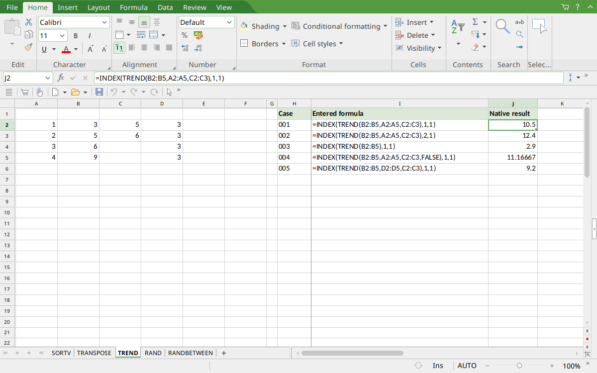
FreeOffice PlanMaker 2024 rev F1238.1005: selected J2 contains =INDEX(TREND(B2:B5,A2:A5,C2:C3),1,1) and displays 10.5. The valid predictions and separate constant-x observation are visible.
Version and evidence scope
Official FreeOffice PlanMaker 2024 reference, checked October 18, 2026. No introduction release is inferred from current support.
Selected examples were tested on October 18, 2026 in FreeOffice PlanMaker 2024 rev F1238.1005, 64-bit. The actual observations are distinguished from independent mathematical references and from teaching extensions not individually executed. Proprietary implementation code has not been inspected. Scalar INDEX readbacks do not establish array-entry or automatic-spill behavior.