Create an ONLYOFFICE Pivot Table and Include New Rows

If new rows are outside a pivot’s source range, refreshing the old range will not include them. Check Show advanced settings → Data Source, extend the range to the last record, then refresh and compare the totals.

Requirements and sample

Use an editable workbook in the current desktop-style ONLYOFFICE Spreadsheet Editor. The steps follow current English help; the bounded native example below was checked in Desktop Editors Community 10.0.0.169. Historical builds and the mobile app are not covered. Save a working copy as XLSX; CSV contains only values and cannot retain a pivot table. The Pivot Table ribbon can be contextual in newer layouts; the Insert tab also documents pivot-table insertion.

Download the eight-row sales CSV. Open it as comma-separated text, verify that Amount contains numbers, and name its worksheet Sales. The data occupies A1:C9:

Region	Channel	Amount
North	Online	120
North	Retail	80
South	Online	90
South	Retail	140
North	Online	60
South	Online	30
North	Retail	40
South	Retail	20

Keep headers on row 1 and exclude blank separators or manually added total rows from the source.

Create the original summary

1. Select the source range and choose Insert → Pivot Table, the route tested in Desktop Editors 10.0.0.169. The contextual Pivot Table ribbon appears after creating or selecting a pivot; other documented layouts may expose Pivot Table → Insert Table.
2. In the creation dialog, confirm the source is Sales!$A$1:$C$9. Choose a new worksheet.
3. In the right-sidebar field areas, place Region in Rows, Channel in Columns, and Amount in Values. Set the Amount summary to Sum.
4. Compare against the independent target below.

Region	Online	Retail	Total
North	180	120	300
South	120	160	280
Grand total	300	280	580

These totals preserve the original eight-record example: North/Online is 120 + 60; South/Retail is 140 + 20. =SUM(C2:C9) on Sales gives 580. See SUM and, for a category-by-category check, SUMIFS.

The creation, field placement and value aggregation are documented in the official pivot guide; the alternative insertion route is in Insert tab help.

Reproduce the missing-row problem

Append these records without inserting rows inside the original range:

Worksheet row	Region	Channel	Amount
10	North	Online	50
11	South	Retail	70

The full source now totals 700: 580 + 50 + 70. A source still ending at C9 covers only the original eight records. Refreshing that unchanged source is expected to leave the pivot at 580. If your particular workbook expands its source automatically, inspect the resulting range and proceed directly to the 700 checks; do not manufacture a failure to match the exercise.

Expand the source, then refresh

1. Select the pivot, open its right-sidebar Show advanced settings, and choose Data Source.
2. Inspect Data Range. Use its range-selection control to change Sales!$A$1:$C$9 to Sales!$A$1:$C$11. Confirm the range dialog and advanced settings.
3. With the pivot selected, click Refresh. Compare every subtotal with the target below, not only the grand total. In the tested build, confirming the expanded source already updated the totals; the explicit Refresh then retained them. This observed behavior does not remove the need to check the source and totals.

The official advanced-settings and refresh instructions document range changes and refresh as distinct operations.

Region	Online	Retail	Total
North	230	120	350
South	120	230	350
Grand total	350	350	700

For a second check, edit the existing C2 amount from 120 to 125, with the expanded source retained. Refresh should now yield North/Online 235, North total 355 and grand total 705. This change is inside the source; it tests updating existing values rather than adding rows. Restore C2 to 120 and refresh again to return to 700.

Diagnose a remaining mismatch

• Still 580: recheck the actual pivot’s Data Source, including the sheet name and final row. There may be several pivots in the workbook.
• 8 or 10 instead of money totals: inspect Values aggregation and numeric import. Count is a different question from Sum.
• Missing category despite C11 being included: examine the pivot’s own filters and slicers. A full source does not mean all categories are displayed.
• Nearly identical categories: compare source labels for spaces or spelling variations before changing the summary.
• Inflated total: check for duplicated imports or a manual total row included as a record.
• Formatted-table source: ONLYOFFICE supports building a pivot from a formatted table, but verify that table’s boundaries and the pivot’s source after appending. This guide makes no universal promise of automatic source expansion.

Retain the original pivot layout when troubleshooting. Rebuilding a simple pivot on a new sheet is a useful comparison if its source settings remain confusing; keep the old one until totals agree.

Native example and test limits

The supplied eight-row CSV was opened as UTF-8, comma-separated data in ONLYOFFICE Desktop Editors Community 10.0.0.169 (x64 deb) on Linux x86_64, with English UI, on October 16, 2026. Numeric Amount checks returned COUNT 8 and SUM 580. The native pivot matched every initial subtotal above.

After appending rows 10 and 11, refreshing the unchanged Sales!$A$1:$C$9 source left the pivot at 580, while the full source summed to 700. Explicitly expanding Data Source to row 11 immediately rebuilt the pivot to 700; a subsequent Refresh retained the expected subtotals. Changing existing C2 to 125 left the pivot at 700 until Refresh, which produced 705, North/Online 235 and North total 355. Restoring C2 to 120 and refreshing returned the pivot to 700.

XLSX save, close and reopen preserved all expanded subtotals and the source ending at C11. The reopened Data range field displayed Sales!A1:C11, without dollar markers; it still referred to the same saved range.

Select a screenshot to open the full-size image.

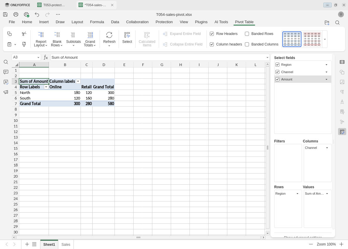
The original eight-row pivot matches the independently calculated 580 summary.

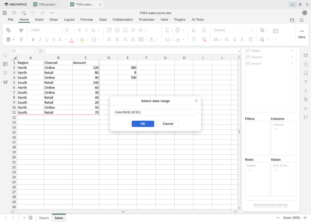
Extend the source through row 11; the diagnostic values in column E are outside the pivot source.

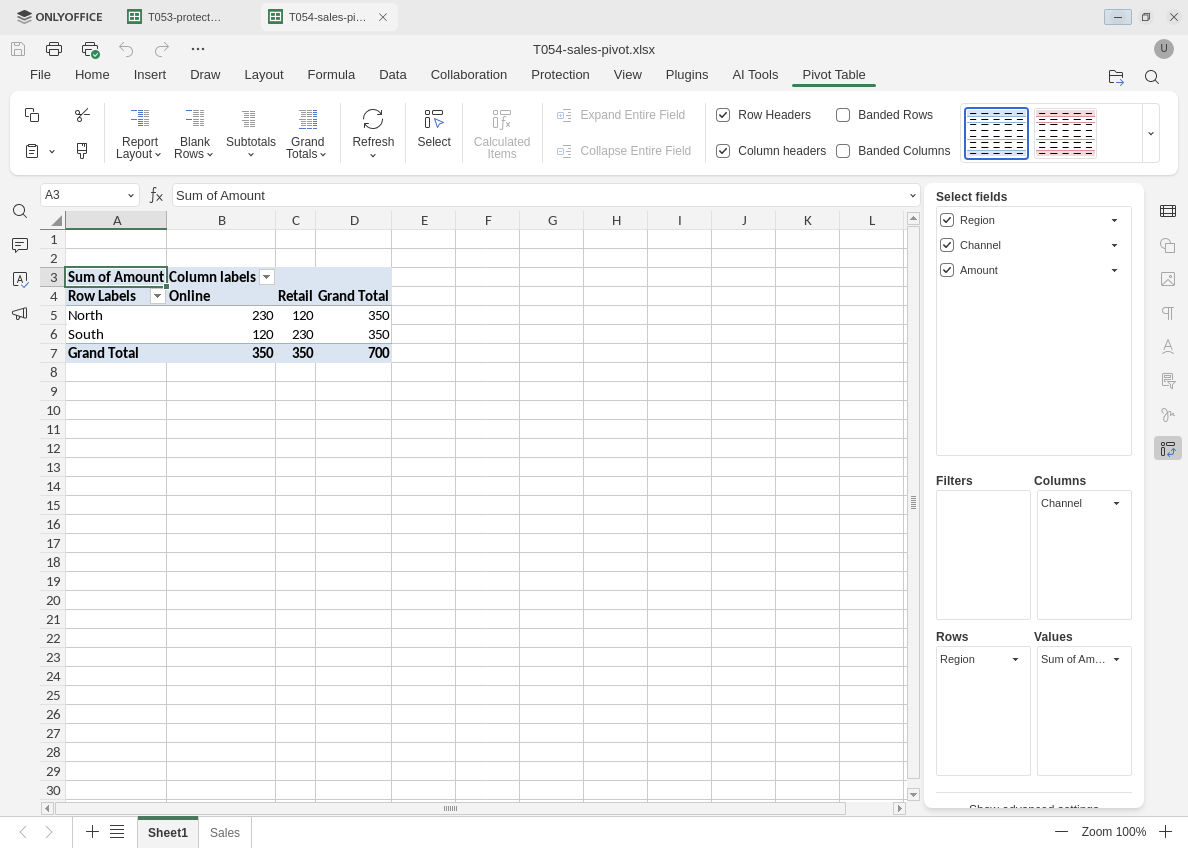
After save and reopen, all expanded subtotals remain correct.

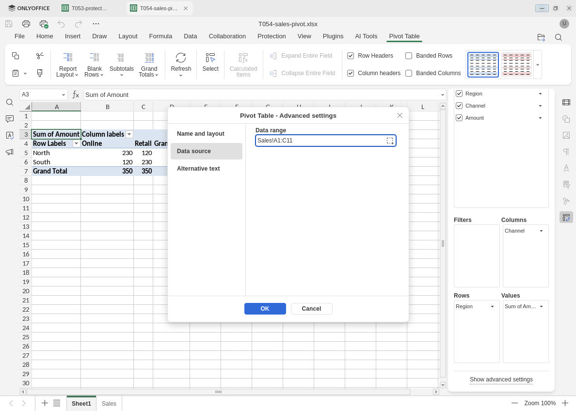
The persisted Data range still ends at C11, although this reopened display omits dollar markers.

Evidence and limits: Official documentation and independently calculated totals were checked separately from native execution. Screenshots are genuine, unmodified captures. This test covered an ordinary fixed cell range, numeric CSV input, Sum aggregation, source expansion, an existing-value refresh and XLSX persistence. Formatted-table or named-range growth, external sources, alternate aggregations, filters/slicers, malformed data, multiple pivots, hosted/mobile builds and other editors were not tested. The existing-value edit was not repeated after reopening; the saved expanded range and 700 outputs were checked.