

ONLYOFFICE PERCENTILE: Interpolation, Endpoints and Response-Time Examples
Use ONLYOFFICE PERCENTILE and its PERCENTILE.INC alias with complete numeric datasets, interpolation examples and separate name-version history.
Verification status: See the evidence and test scope described in this guide. How formula examples are checked
PERCENTILE returns a value at a chosen percentile of a numeric dataset. The probability input is a fraction: 0.9 means the 90th percentile, whereas 90 is outside the documented range. A percentile is a value in the data’s units, not a percentage result.
Availability and version history
- Introduced: PERCENTILE’s original introduction is unknown. The Desktop changelog adds its PERCENTILE.INC alias in 4.4.1; Docs/mobile introduction dates remain unknown.
- Availability: Documented in current ONLYOFFICE Spreadsheet Editor help; no final supported-version endpoint is established.
- Scope: Desktop and Docs release separately. The checked source revision does not establish identical behavior on every deployment, mobile client or older build.
- Checked: October 14, 2026, against the official PERCENTILE reference, vendor illustration and pinned source. Worked outputs were independently calculated; no native percentile test was performed.
Syntax and inclusive endpoints
PERCENTILE(array, k)
The official reference takes a selected data range and a numeric k from 0 through 1, inclusive. Both arguments are supplied. The short help entry does not specify an omitted-argument default or a complete mixed-type/error table.
For the complete numeric examples below, the pinned official calculation source sorts the values and interpolates between adjacent observations. With n observations, the one-based position is h=1+(n−1)k. An integer h selects that observation; otherwise the fractional part describes progress from the lower observation to the next. This is source-backed reconstruction, not a native test or a promise about every installed build.
Reproduce the vendor’s complete grid
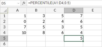
On a new VendorPercentile sheet, enter this grid in A1:D4, without headers inside it:
| Row | A | B | C | D |
|---|---|---|---|---|
| 1 | 1 | 3 | 5 | 7 |
| 2 | 0 | 2 | 4 | 6 |
| 3 | 7 | 5 | 3 | 5 |
| 4 | 10 | 8 | 6 | 4 |
Put =PERCENTILE(A1:D4,0.5) in D5, outside the selected input. The official illustration shows 5. Independently sorting the sixteen values puts 5 in both the eighth and ninth positions, so their midpoint is also 5. The screenshot is vendor evidence, not a screenshot from a new local run.
Calculate percentiles of eight response times
Create ResponseTimes, reserving A1:H12. Put Minutes in A1 and enter 12,15,18,18,22,27,35,45 in A2:A9. Each is one measured response time; retain both 18s as separate observations.
Put Probability in C1 and Percentile minutes in D1. Enter these k values in C2:C8. In D2 put =PERCENTILE($A$2:$A$9,C2) and fill through D8.
| Row | C: k | Expected D: minutes |
|---|---|---|
| 2 | 0 | 12 |
| 3 | 0.25 | 17.25 |
| 4 | 0.5 | 20 |
| 5 | 0.6 | 23 |
| 6 | 0.75 | 29 |
| 7 | 0.9 | 38 |
| 8 | 1 | 45 |
Put =COUNT(A2:A9) in G2 for 8, =MIN(A2:A9) in G3 for 12, and =MAX(A2:A9) in G4 for 45. The count is a control for these explicit numeric inputs; it does not settle unusual mixed-type handling.
The 25th-percentile position is 1+7×0.25=2.75, between the second value 15 and third value 18. In G6 enter =15+0.75*(18-15) for 17.25. The median lies between the fourth and fifth values, giving (18+22)/2=20. The 90th-percentile position is 7.3, giving 35+0.3×(45−35)=38.
Advanced: change the origin without changing relative spacing
Copy ResponseTimes as OffsetTimes. Replace A2:A9 with 72,75,78,78,82,87,95,105, adding 60 to every original observation. Leave C unchanged; the existing D formulas now have expected results 72,77.25,80,83,89,98,105.
G2 remains 8, while G3/G4 become 72/105. Update the hand control in G6 to =75+0.75*(78-75) for 77.25 so it describes the copied data too.
Each percentile increased by 60. The ordering and fractional interpolation weights stayed the same. A different zero point changes the reported values without changing the spacing between observations; it does not multiply the percentile probability.
PERCENTILE.INC alias and name availability
The official PERCENTILE.INC reference documents the same two arguments and inclusive probability endpoints as PERCENTILE. In the pinned source, the .INC name directly inherits the legacy calculation and argument contract; only its name/registration metadata differs. Both documented names are covered here, while PERCENTILE.EXC remains a separate convention.
The Desktop Editors changelog explicitly adds PERCENTILE.INC in version 4.4.1. The original PERCENTILE introduction and either name’s Docs/mobile introduction remain unknown. Both names are currently documented; the alias is not a retirement notice.
On VendorPercentile, put =PERCENTILE.INC(A1:D4,1) in F5. The separate INC illustration shows 10, the maximum of that complete grid. Its probability is 1, whereas the earlier legacy screenshot asks for 0.5.

Build the five-invoice worksheet
Create InvoicePercentiles, reserving A1:H12. Put Amount in A1 and enter 80,120,150,210,400 in A2:A6. All values use the same currency and reporting basis; the currency symbol is display formatting rather than an extra argument.
Put Probability, Inclusive amount and Legacy comparison in C1:E1. Enter the probabilities below in C2:C8. In D2 put =PERCENTILE.INC($A$2:$A$6,C2) and in E2 put =PERCENTILE($A$2:$A$6,C2). Fill both through row 8.
| Row | C: k | Expected D and E |
|---|---|---|
| 2 | 0 | 80 |
| 3 | 0.1 | 96 |
| 4 | 0.25 | 120 |
| 5 | 0.5 | 150 |
| 6 | 0.75 | 210 |
| 7 | 0.9 | 324 |
| 8 | 1 | 400 |
Put =D2-E2 in F2 and fill through F8 for seven expected zeros. These comparisons check the relationship for this numeric fixture, rather than every possible input type.
For k=0.1, h=1.4 and the amount is 80+0.4×(120−80)=96. For k=0.9, h=4.6 and the amount is 210+0.6×(400−210)=324. Put those two hand calculations in H2 and H3, using =80+0.4*(120-80) and =210+0.6*(400-210).
Advanced: inspect sensitivity to one large invoice
Copy InvoicePercentiles as LargerFinalInvoice and change A6 from 400 to 1000. Leave the probability column unchanged. The expected D/E sequence is now 80,96,120,150,210,684,1000; F2:F8 still contains zeros.
H2 remains 96. Update H3 to =210+0.6*(1000-210) for 684. The 600-unit increase in the last observation increases the 90th percentile by 360, because its interpolation gives that endpoint a 0.6 weight. The median and 75th percentile remain 150 and 210.
The result is neither immune to an extreme value nor equal to that value. Its sensitivity depends on the requested position and the neighboring observations. Preserve the original sheet to distinguish a real changed measurement from a different percentile convention.
A percentile need not be an observed invoice
Neither 96 nor 324 occurs in the original five-value register. They are interpolated amounts. Four of five invoices are at or below 324, so the observed fraction is 80% even though the requested percentile probability is 90%.
If a report must return an actual invoice amount at a particular ordered position, LARGE or SMALL answers that different question. If it must identify the associated invoice, the value alone is insufficient, especially when amounts repeat.
Interpret the cutoff correctly
In the original ResponseTimes data, seven of eight observations are at or below 38 minutes. That is 87.5%, not exactly 90%. Interpolation can place a percentile between measured values; it does not manufacture extra observations to make an empirical count equal the requested probability.
The result also does not establish that 90% of future response times will fall below 38. It summarizes this selected sample under the stated convention. Specify whether you want an interpolated percentile, an actual ordered observation, or a count below an operational threshold.
PERCENTILE.INC shares the legacy implementation in the pinned source. PERCENTILE.EXC uses a different position convention and sample-dependent limits; swapping names can change the result.
Boundaries and troubleshooting
Use numeric k within the documented domain and keep headers outside the data range. Blank cells, text, Boolean values, errors and numeric strings can change the effective input set; their native handling is not established by these all-numeric examples. Do not assume that every blank-looking cell means missing data, or replace missing observations with zero without considering its meaning.
The calculations use scalar formulas, ordinary numeric ranges and English comma separators. They do not establish array-spill behavior, extreme precision, invalid-input error tokens or workbook round-trip parity. COUNT, MIN and MAX help check this fixture’s size and endpoints, without acting as a universal validation rule.